Exploring #SOTEU speeches
Giorgio Comai (OBC Transeuropa/#edjnet)
13 September 2017
This post offers different examples of data visualisation aimed at exploring “State of the Union” speeches since they have first been introduced in 2010 (the speech was not delivered in 2014 because of European Parliament elections). It highlights key steps in the procedure, and includes the actual code in the R programming language used to create them (hidden by default).
The source document can be downloaded from GitHub.
Downloading the speeches
The full transcript of the speeches is available on the official website of the European Union. Here are the direct links to each of the speeches:
# introduce links to speeches
links <- tribble(~Year, ~President, ~Link,
2010, "Barroso", "http://europa.eu/rapid/press-release_SPEECH-10-411_en.htm",
2011, "Barroso", "http://europa.eu/rapid/press-release_SPEECH-11-607_en.htm",
2012, "Barroso", "http://europa.eu/rapid/press-release_SPEECH-12-596_en.htm",
2013, "Barroso", "http://europa.eu/rapid/press-release_SPEECH-13-684_en.htm",
2015, "Juncker", "http://europa.eu/rapid/press-release_SPEECH-15-5614_en.htm",
2016, "Juncker", "http://europa.eu/rapid/press-release_SPEECH-16-3043_en.htm",
2017, "Juncker", "http://europa.eu/rapid/press-release_SPEECH-17-3165_en.htm")
# store html files locally
dir.create(path = "html_soteu", showWarnings = FALSE)
dir.create(path = file.path("img"), showWarnings = FALSE)
# add local link to data.frame
links <- dplyr::bind_cols(links, data_frame(LocalLink = file.path("html_soteu", paste0(links$Year, "-", links$President, ".html"))))
for (i in seq_along(along.with = links$Link)) {
if (file.exists(links$LocalLink[i]) == FALSE) { # download files only if not previously downloaded
download.file(url = links$Link[i], destfile = links$LocalLink[i])
Sys.sleep(time = 1)
}
}
knitr::kable(links)| Year | President | Link | LocalLink |
|---|---|---|---|
| 2010 | Barroso | http://europa.eu/rapid/press-release_SPEECH-10-411_en.htm | html_soteu/2010-Barroso.html |
| 2011 | Barroso | http://europa.eu/rapid/press-release_SPEECH-11-607_en.htm | html_soteu/2011-Barroso.html |
| 2012 | Barroso | http://europa.eu/rapid/press-release_SPEECH-12-596_en.htm | html_soteu/2012-Barroso.html |
| 2013 | Barroso | http://europa.eu/rapid/press-release_SPEECH-13-684_en.htm | html_soteu/2013-Barroso.html |
| 2015 | Juncker | http://europa.eu/rapid/press-release_SPEECH-15-5614_en.htm | html_soteu/2015-Juncker.html |
| 2016 | Juncker | http://europa.eu/rapid/press-release_SPEECH-16-3043_en.htm | html_soteu/2016-Juncker.html |
| 2017 | Juncker | http://europa.eu/rapid/press-release_SPEECH-17-3165_en.htm | html_soteu/2017-Juncker.html |
In order to process them as data, it is necessary to extract first the relevant sections of the webpage.
# extract speeches
tempNodes <- purrr::map(.x = links$LocalLink, .f = function(x) read_html(x)%>% html_nodes("div"))
text <- c( (tempNodes[[1]] %>% html_nodes("td") %>% html_text())[2], # that's because previous pages have their layout built through tables, old styles
(tempNodes[[2]] %>% html_nodes("td") %>% html_text())[2],
(tempNodes[[3]] %>% html_nodes("td") %>% html_text())[2],
(tempNodes[[4]] %>% html_nodes("td") %>% html_text())[2],
tempNodes[[5]] %>% html_nodes(".content") %>% html_text(), # selecting the relevant div
tempNodes[[6]] %>% html_nodes(".content") %>% html_text(),
tempNodes[[7]] %>% html_nodes(".content") %>% html_text()
)The same could effectively be accomplished by copy/pasting the transcripts.
Word substitutions
In order to analyse texts, it is common to stem words to ensure that “example” and “examples” are counted as one and the same word. Rather than stemming all words (which would make some of them unclear in the graphs that follow), only selected keywords are stemmed (e.g. ‘citizens’ is transformed to ‘citizen’, and ‘refugees’ is transformed to ‘refugee’). Self-referential words such as ‘european’, ‘commission’, ‘union’, and ‘eu’ are excluded from the following graphs: they are found much more frequently than all others and would effectively obscure more interesting results. Stopwords such as ‘and’, ‘also’, and ‘or’ are also excluded.
text <- gsub(pattern = "refugees", replacement = "refugee", x = text)
text <- gsub(pattern = "citizens", replacement = "citizen", x = text)
exclude <- data_frame(word = c("european", "europe", "union", "commission", "eu", "means"))
speechesOriginal <- bind_cols(id = paste(links$President, links$Year), links, txt = text)
speechesOriginal_byWord <- speechesOriginal %>% unnest_tokens(word, txt, to_lower = TRUE)
speeches <- speechesOriginal %>%
unnest_tokens(word, txt, to_lower = TRUE) %>%
anti_join(stop_words) %>% # removing a standard list of stopwords
anti_join(exclude) # remove selected keywords
speeches_by_speech <- speeches %>%
anti_join(stop_words) %>% # removes stop words
group_by(id, word) %>% # makes sure wordcount is calculated on a per speech basis
count(word, sort = TRUE) %>% # counts words
group_by(word) %>%
mutate(total = (sum(n))) %>% # counts total number of occurrences of every word in all speeches
arrange(total) %>% # orders data by total number of occurrences
ungroup()
# this exports the documents as extracted; useful to check if the text has been imported correctly
writeLines(paste("Speech:", unique(speeches$id), "\n", text, " ___ ______ ______ ______ ______ ______ ______ ______ ______ ___\n __)(__ __)(__ __)(__ __)(__ __)(__ __)(__ __)(__ __)(__ __)(__\n (______)(______)(______)(______)(______)(______)(______)(______)(______)\n", sep = "\n"), file.path("allSpeeches.txt"))Not all #SOTEU have the same length
In particular, the fact that the speech Juncker gave in 2015 was substantially lenghtier than the others should be kept in consideration when looking at some of the figures below.
knitr::kable(speechesOriginal_byWord %>% group_by(id) %>% count())| id | n |
|---|---|
| Barroso 2010 | 4381 |
| Barroso 2011 | 4977 |
| Barroso 2012 | 6108 |
| Barroso 2013 | 5658 |
| Juncker 2015 | 10056 |
| Juncker 2016 | 6041 |
| Juncker 2017 | 6130 |
speechesOriginal_byWord %>% group_by(id) %>% count() %>%
ggplot(mapping = aes(x = id, y = n)) +
geom_col() +
scale_x_discrete(name = "") +
scale_y_continuous(name = "") +
theme_minimal() +
labs(title = "Number of words for each #SOTEU")
ggsave(file.path("img", "number of words in each SOTEU.png"))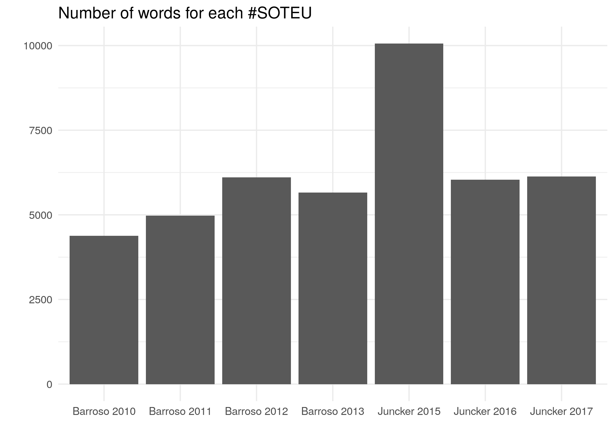
What are the most frequent keywords across all speeches
Here are different ways to look at the words most frequently found in all SOTEU speeches.
mostFrequent_barchart_20 <-
speeches_by_speech %>%
group_by(word) %>%
arrange(desc(total)) %>%
group_by(id) %>%
top_n(20) %>%
arrange(total) %>%
mutate(word = factor(word, levels = unique(word))) %>% # makes sure order is kept for graph
ggplot(mapping = aes(x = word, y = n, label = n, fill = total)) +
geom_col() +
scale_x_discrete(name = "") +
scale_y_continuous(name = "") +
scale_fill_continuous(low = "yellow", high = "red") +
coord_flip() +
theme_minimal() +
labs(title = "Most frequent keywords in all #SOTEU speeches", fill = "Word frequency", caption = "Data processing: Giorgio Comai / OBC Transeuropa / #edjnet")
mostFrequent_barchart_20
ggsave(filename = file.path("img", "mostFrequent_barchart_20.png"), plot = mostFrequent_barchart_20)Download this graph in png format.
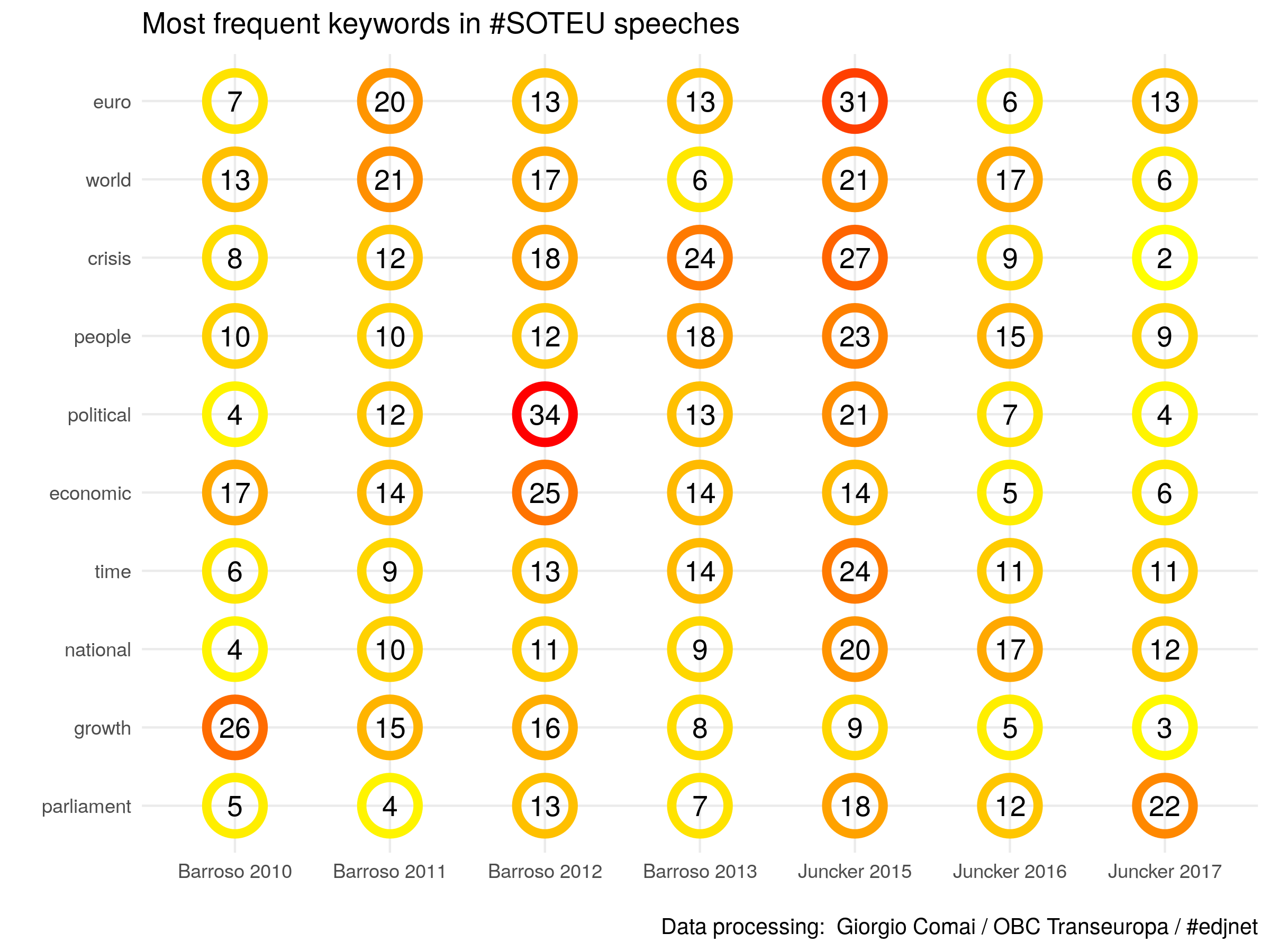
keywords_circles_mostFrequent <- speeches_by_speech %>%
group_by(word) %>%
arrange(desc(total)) %>%
group_by(id) %>% top_n(10) %>%
arrange(total) %>%
mutate(word = factor(word, levels = unique(word))) %>% # makes sure order is kept for graph
ggplot(mapping = aes(x = word, y = id, size = n, colour = n, label = n)) +
geom_point(shape = 21, stroke = 3, size = 10) +
geom_text(mapping = aes(size = 25), colour = "black") +
scale_colour_continuous(low = "yellow", high = "red")+
scale_x_discrete(name = "") +
scale_y_discrete(name = "") +
coord_flip() +
theme_minimal() +
theme(legend.position="none") +
labs(title = "Most frequent keywords in #SOTEU speeches", caption = "Data processing: Giorgio Comai / OBC Transeuropa / #edjnet")
keywords_circles_mostFrequent
ggsave(filename = file.path("img", "keywords_circles_mostFrequent.png"), plot = keywords_circles_mostFrequent, width = 8, height = 6)Download this graph in png format.
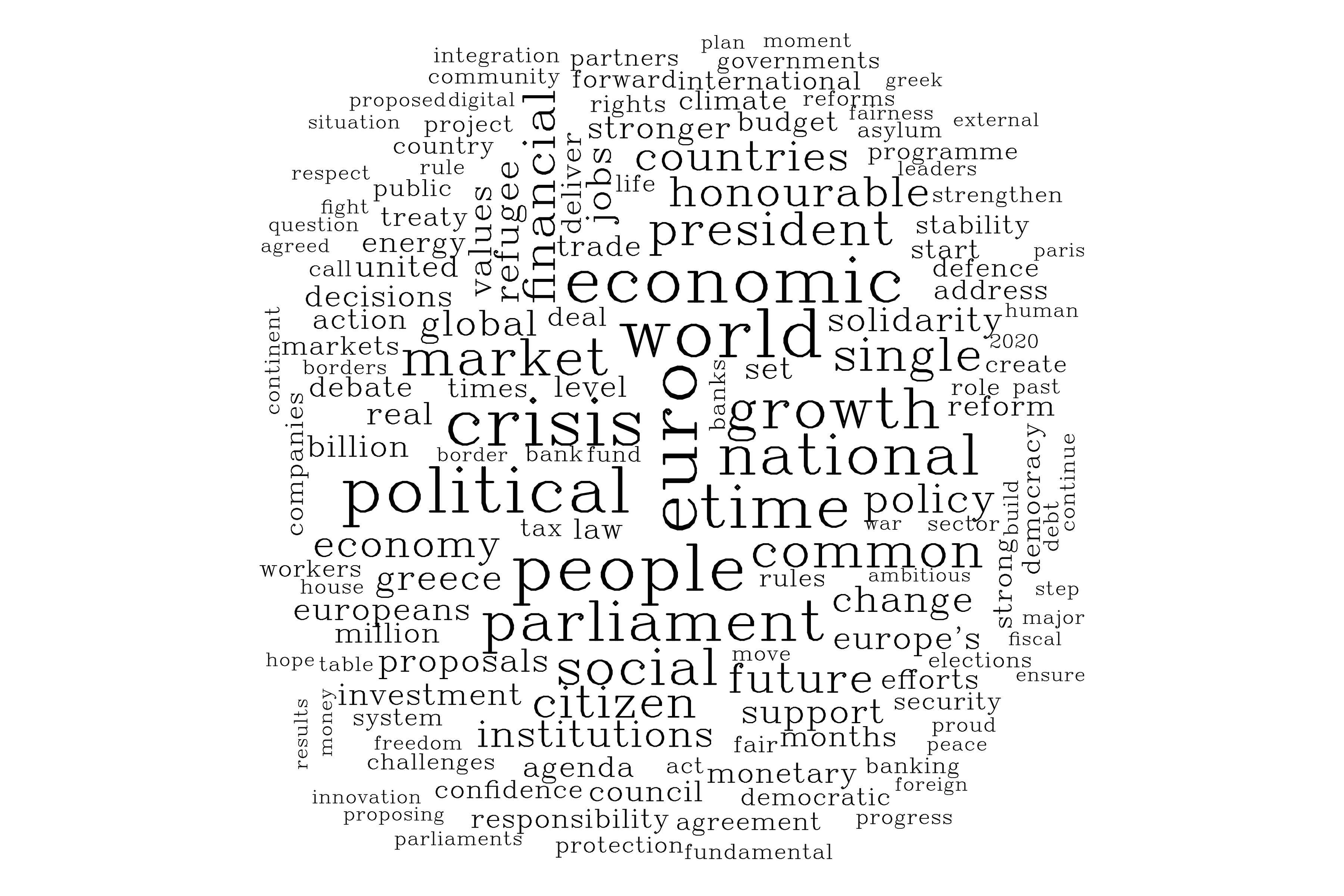
speeches %>%
anti_join(stop_words) %>%
count(word) %>%
with(wordcloud(word, n, max.words = 150,
random.order = FALSE,
random.color = FALSE,
colors = TRUE, vfont=c("serif","plain")))
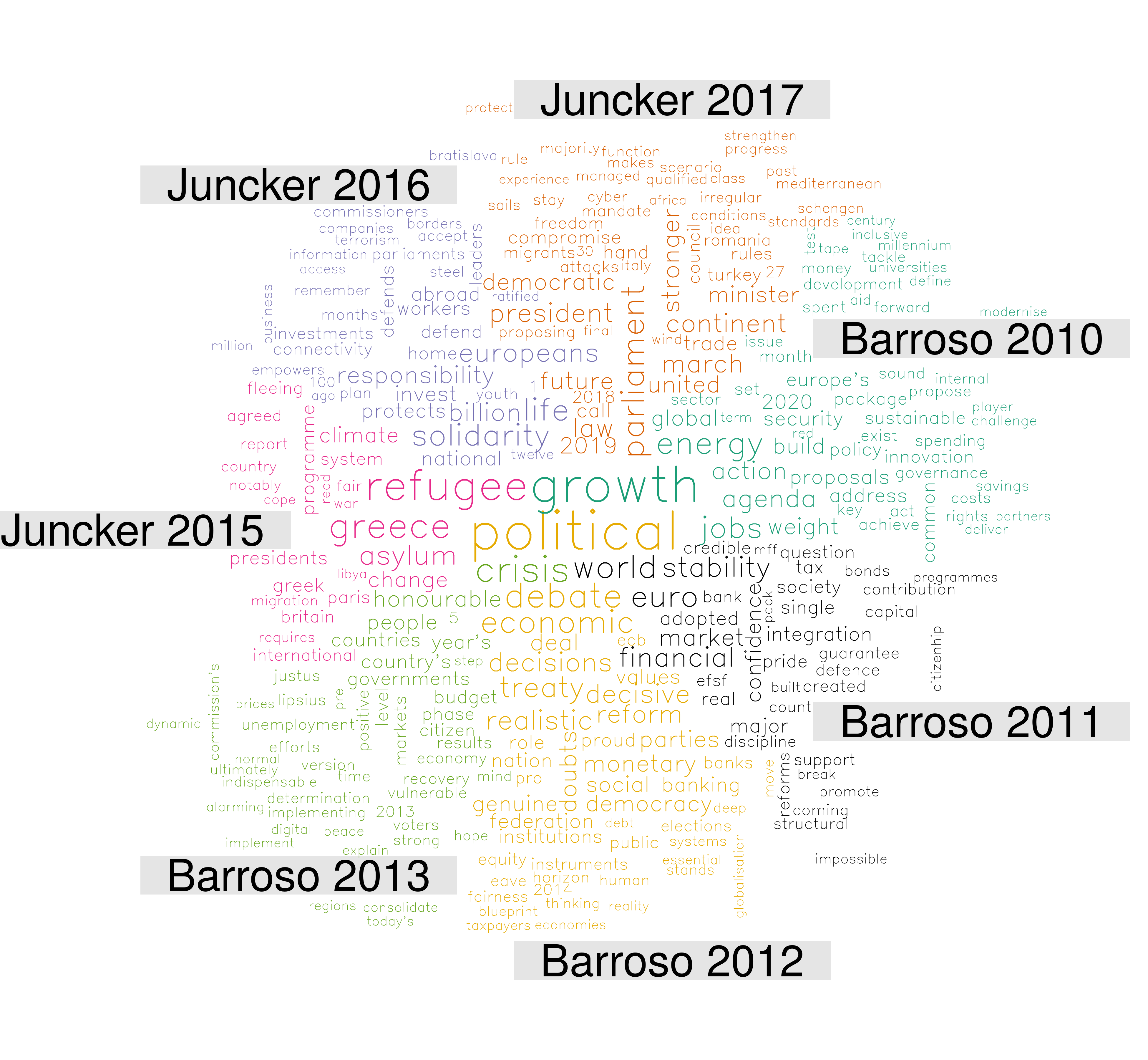
What are the most distinctive words of each SOTEU speech?
The following wordcloud compares the frequency of words across speeches, showing the words that are most frequent in each of the speech and are at the same time less frequently found in other speeches.
speeches %>%
anti_join(stop_words) %>%
group_by(id) %>%
count(word) %>%
arrange(desc(id)) %>%
spread(id, n) %>%
select(word, `Barroso 2010`, `Juncker 2017`, `Juncker 2016`, `Juncker 2015`, `Barroso 2013`, `Barroso 2012`, `Barroso 2011`) %>%
remove_rownames() %>%
column_to_rownames("word") %>%
replace(is.na(.), 0) %>%
comparison.cloud(max.words = 300, colors=brewer.pal(6, "Dark2"),
vfont=c("sans serif","plain"))
Selected keywords
keywords_circles <- speeches_by_speech %>%
filter(word == "solidarity" | word == "refugee" |word == "crisis" | word == "greece"| word == "climate" | word == "citizens"| word == "euro" | word == "jobs" ) %>%
mutate(word = factor(word, levels = unique(word))) %>% # makes sure order is kept for graph
ggplot(mapping = aes(x = word, y = id, size = n, colour = n, label = n)) +
geom_point(shape = 21, stroke = 3, size = 10) +
geom_text(mapping = aes(size = 25), colour = "black") +
scale_colour_continuous(low = "yellow", high = "red")+
scale_x_discrete(name = "") +
scale_y_discrete(name = "") +
coord_flip() +
theme_minimal() +
theme(legend.position="none") +
labs(title = "Frequency of selected keywords in #SOTEU speeches")
keywords_circles
ggsave(filename = file.path("img","keywords_circles.png"), plot = keywords_circles)
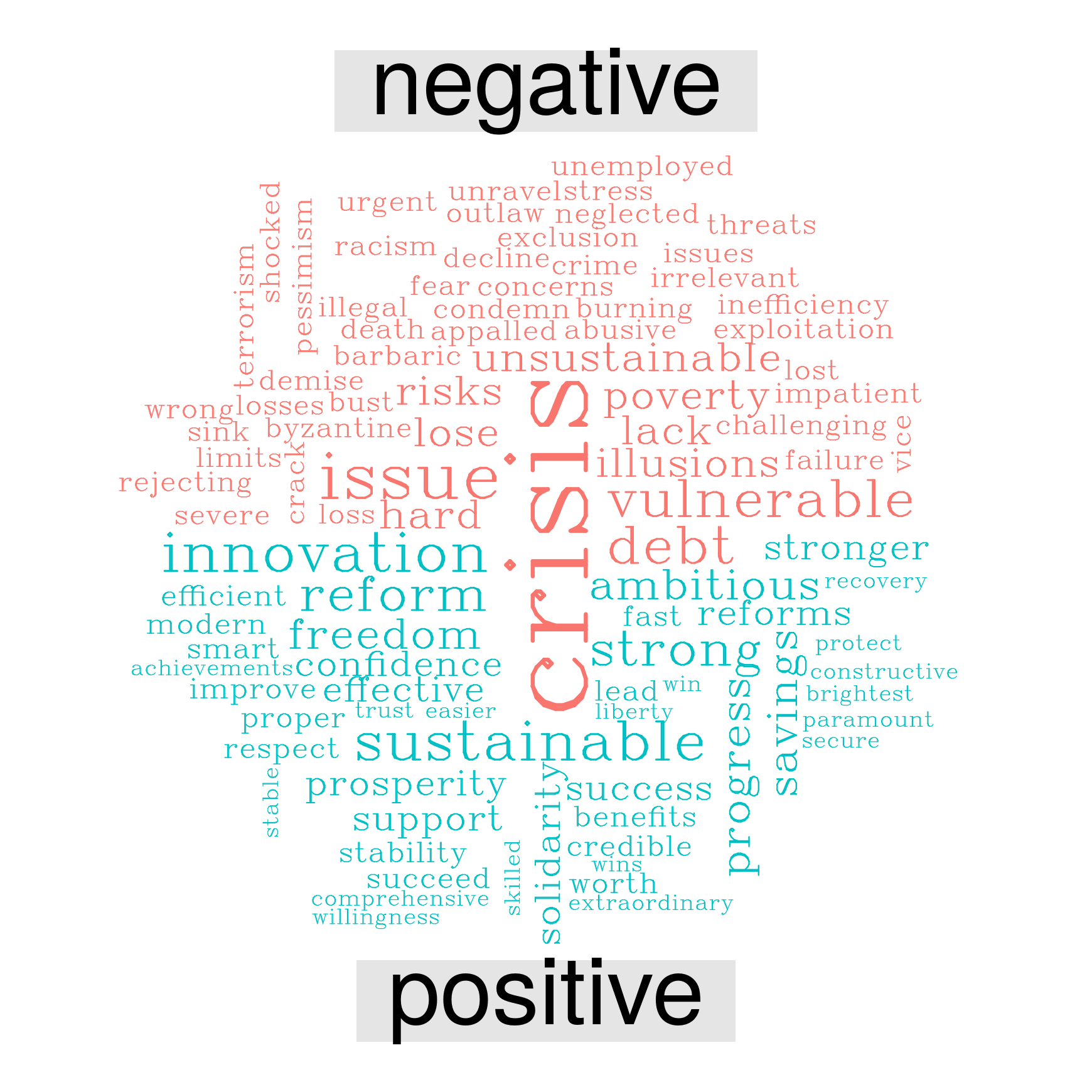
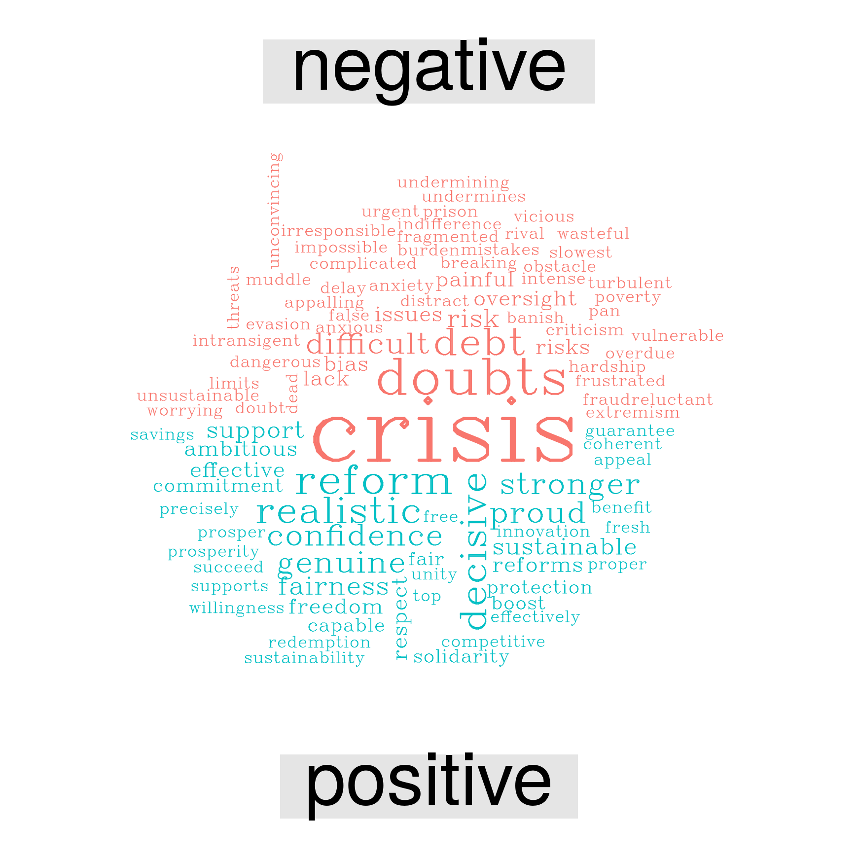
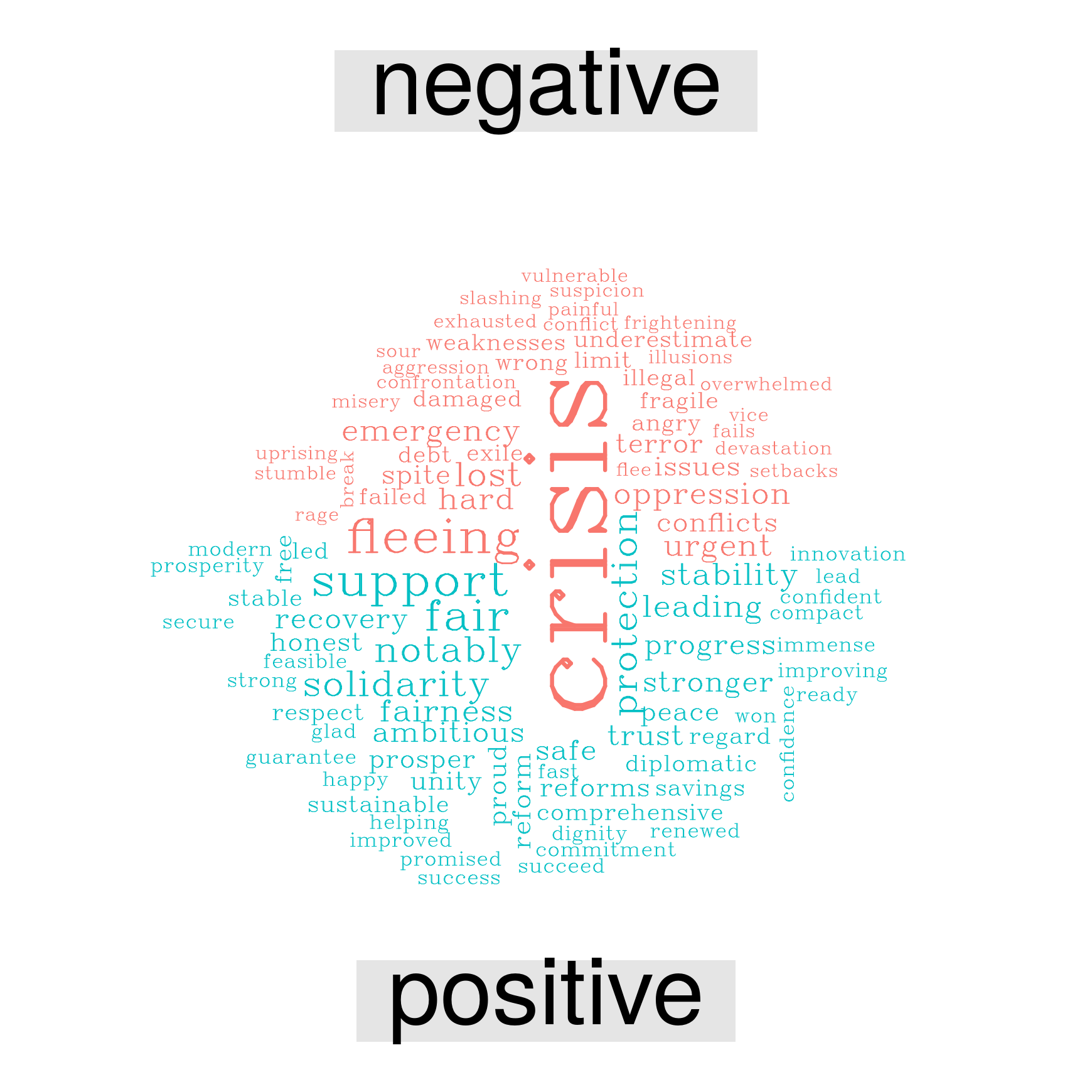
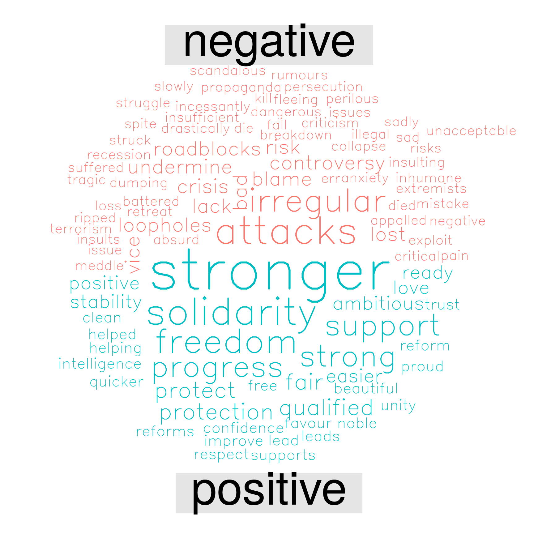
Words with positive/negative connotation
The following wordclouds highlight the frequency of words which have a positive and negative connotation according to the lexicon by Bing Liu and collaborators.1
Looking at these wordlcouds, it quickly appears that ‘crisis’ is the dominant negative words in each of the speeches, but the positive counterpoint is different every year.
All speeches
speeches %>%
inner_join(get_sentiments("bing")) %>%
count(word, sentiment, sort = TRUE) %>%
acast(word ~ sentiment, value.var = "n", fill = 0) %>%
comparison.cloud(colors = c("#F8766D", "#00BFC4"),
max.words = 100, vfont=c("serif","plain"))
Barroso 2010
speeches %>%
filter(id == "Barroso 2010") %>%
inner_join(get_sentiments("bing")) %>%
count(word, sentiment, sort = TRUE) %>%
acast(word ~ sentiment, value.var = "n", fill = 0) %>%
comparison.cloud(colors = c("#F8766D", "#00BFC4"),
max.words = 100, vfont=c("serif","plain"))
Barroso 2011
speeches %>%
filter(id == "Barroso 2011") %>%
inner_join(get_sentiments("bing")) %>%
count(word, sentiment, sort = TRUE) %>%
acast(word ~ sentiment, value.var = "n", fill = 0) %>%
comparison.cloud(colors = c("#F8766D", "#00BFC4"),
max.words = 100, vfont=c("serif","plain"))
Barroso 2012
speeches %>%
filter(id == "Barroso 2012") %>%
inner_join(get_sentiments("bing")) %>%
count(word, sentiment, sort = TRUE) %>%
acast(word ~ sentiment, value.var = "n", fill = 0) %>%
comparison.cloud(colors = c("#F8766D", "#00BFC4"),
max.words = 100, vfont=c("serif","plain"))
Barroso 2013
speeches %>%
filter(id == "Barroso 2013") %>%
inner_join(get_sentiments("bing")) %>%
count(word, sentiment, sort = TRUE) %>%
acast(word ~ sentiment, value.var = "n", fill = 0) %>%
comparison.cloud(colors = c("#F8766D", "#00BFC4"),
max.words = 100, vfont=c("serif","plain"))
Juncker 2015
speeches %>%
filter(id == "Juncker 2015") %>%
inner_join(get_sentiments("bing")) %>%
count(word, sentiment, sort = TRUE) %>%
acast(word ~ sentiment, value.var = "n", fill = 0) %>%
comparison.cloud(colors = c("#F8766D", "#00BFC4"),
max.words = 100, vfont=c("serif","plain"))
Juncker 2016
speeches %>%
filter(id == "Juncker 2016") %>%
inner_join(get_sentiments("bing")) %>%
count(word, sentiment, sort = TRUE) %>%
acast(word ~ sentiment, value.var = "n", fill = 0) %>%
comparison.cloud(colors = c("#F8766D", "#00BFC4"),
max.words = 100, vfont=c("sans serif","plain"))
Juncker 2017
speeches %>%
filter(id == "Juncker 2017") %>%
inner_join(get_sentiments("bing")) %>%
count(word, sentiment, sort = TRUE) %>%
acast(word ~ sentiment, value.var = "n", fill = 0) %>%
comparison.cloud(colors = c("#F8766D", "#00BFC4"),
max.words = 100, vfont=c("sans serif","plain"))
License
This document, the graphs, and the code are distributed under a Creative Commons license (BY). In brief, you can use and adapt all of the above as long you acknowledge the source: Giorgio Comai/OBC Transeuropa/#edjnet - https://datavis.europeandatajournalism.eu/obct/soteu/.
Yes, clicking through their webpage feels as if entering a time warp, but Bing Liu’s dictionary is widely used. He recently published ‘Sentiment Analysis: mining sentiments, opinions, and emotions’ with Cambridge University Press.↩